Cheat Sheet For Probability Theory Page 4
ADVERTISEMENT
 1
1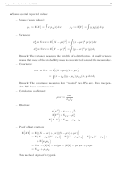 2
2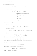 3
3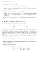 4
4 5
5 6
64
Ingmar Land, October 8, 2005
• The RVs are called uncorrelated if
≡ Σ
= E (X − µ
)(Y − µ
) = 0.
σ
XY
XY
X
Y
Remark: If RVs are independent, they are also uncorrelated. The reverse holds only
for Gaussian RVs (see below).
• Two RVs X and Y are called orthogonal if E[XY ] = 0.
2
Remark: The RVs with finite energy, E[X
] < ∞, form a vector space with scalar
product X, Y
= E[XY ] and norm X
=
E[X
2
]. (This is used in MMSE
estimation.)
These relations for scalar-valued RVs are generalized to vector-valued RVs in the
following.
2
Vector-valued Random Variables
Consider two real-valued vector-valued random variables (RV)
X
Y
1
1
X =
Y =
,
X
Y
2
2
with the individual probability distributions p
(x) and p
(y), and the joint distribution
X
Y
(x, y). (The following considerations can be generalized to longer vectors, of course.)
p
X,Y
The probability distributions are probability mass functions (pmf) if the random vari-
ables take discrete values, and they are probability density functions (pmf) if the random
variables are continuous. Some authors use f () instead of p(), especially for continuous
RVs.
In the following, the RVs are assumed to be continuous. (For discrete RVs, the integrals
have simply to be replaced by sums.)
Remark: The following matrix notations may seem to be cumbersome at the first
glance, but they turn out to be quite handy and convenient (once you got used to).
• Marginal distributions, conditional distributions, Bayes’ rule, expected values work
as in the scalar case.
• Some special expected values:
– Mean vector (vector of mean values):
E[X
]
X
µ
X
1
1
:= E X = E
=
=
µ
1
E[X
]
X
µ
X
X
2
2
2
ADVERTISEMENT
0 votes
Related Articles
Related forms


Related Categories
Parent category: Education