Deriving Relationships From Graphs
ADVERTISEMENT
 1
1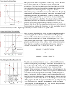 2
2Deriving Relationships from Graphs
Graphing is a powerful tool for representing and interpreting numerical data. In addition, graphs and
knowledge of algebra can be used to find the relationship between variables plotted on a scatter chart.
Consider the following examples and procedures. Become familiar with these approaches, and attempt to
thoroughly understand the processes illustrated here. You will be using these approaches regularly in
introductory physics laboratory activities. Please note that this is merely an introduction to deriving
relationships from graphs. There ultimately will be much more to learn.
Linear Relationships:
The graph to the left depicts a linear relationship. That is,
the data points all can be connected with a straight line.
Note that the best-fit line does not pass through the origin;
rather, it passes through the y-axis at -1m. How would one
define the relationship between the values of the x and y
coordinates in this relationship? It’s done with the equation
of a straight line, y = mx + b where m is the slope and b is
the value of the y-intercept – the value of y when x = 0. The
slope, m, is found from Δy/Δx = (y
- y
)/(x
- x
) = 2m/s in
2
1
2
1
this graph. The value of b can be found from inspection as
equal to -1m. The algebraic relationship is then represented
as y = mx + b where y is identified with the distance, x is
identified with time, m the slope, and b the y-intercept.
Thus, our relationship from the graph is:
distance = (2m/s)time – 1m.
Proportional Relationships:
The graph to the left approximates the proportional
relationship between voltage and current in a circuit. Note
that a relationship is directly proportional only when the
relationship is linear and passes through the origin. This is
not quite the case in the current graph. The value of b is
0.0180 amps. The linear fit derived by the computer used to
generate the graph performs an algebraic best fit to the data.
The equation generated is the best mathematical fit, but the
fit does not properly represent the physical reality of the
situation. If no voltage is applied, then no current flows. If
this is the case, the best-fit line must pass through the origin
in what is known as a physical fit of the data. A physical fit
demands y = Ax as the model for the fit. Under the new
analysis m = 2amps/volt. Then we find:
current = (2amps/volt)voltage
(continued)
ADVERTISEMENT
0 votes
Related Articles
Related forms


Related Categories
Parent category: Business