The Ultimate R Cheat Sheet - Data Management printable pdf download

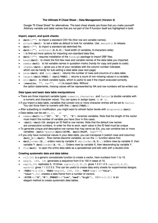
The Ultimate R Cheat Sheet – Data Management (Version 4)

Google “R Cheat Sheet” for alternatives. The best cheat sheets are those that you make yourself!

Arbitrary variable and table names that are not part of the R function itself are highlighted in bold.

Import, export, and quick checks



dat1=read.csv("name.csv") to import a standard CSV file (first row are variable names).



attach(dat1) to set a table as default to look for variables. Use detach() to release.



dat1=read.delim("name.txt") to import a standard tab-delimited file.



dat1=read.fwf("name.prn", widths=c(8,8,8)) fixed width (3 variables, 8 characters wide).



?read.table to find out more options for importing non-standard data files.



dat1=read.dbf("name.dbf") requires installation of the foreign package to import DBF files.



head(dat1) to check the first few rows and variable names of the data table you imported.



names(dat1) to list variable names in quotation marks (handy for copy and paste to code).



data.frame(names(dat1)) gives you a list of your variables with the column number indicated,

which can be handy for sub-setting a data table (see next page)



nrow(dat1) and ncol(dat1) returns the number of rows and columns of a data table.



length(dat1$VAR1[!is.na(dat1$VAR1)] returns a count of non-missing values in a variable.



str(dat1) to check variable types, which is useful to see if the import executed correctly.



write.csv(results, "myresults.csv", na="", row.names=F) to export data. Without

the option statements, missing values will be represented by NA and row numbers will be written out.

Data types and basic data table manipulations



There are three important variable types: numeric, character and factor (a double variable with

a numeric and character value). You can query or assign types: is.factor() or as.factor().



If you import a data table, variables that contain one or more character entries will be set to factor.

You can force them to numeric with this: as.numeric(as.character(dat1$VAR1))



After subsetting or modification, you might want to refresh factor levels with droplevels(dat1)



Data tables can be set as.data.frame(), as.matrix(), as.distance()



names(dat1)=c("ID", "X", "Y", "Z") renames variables. Note that the length of the vector

must match the number of variable you have (four in this case).



row.names(dat1)=dat1$ID. assigns an ID field to row names. Note that the default row names

are consecutive numbers. In order for this to work, each value in the ID field must be unique.



To generate unique and descriptive row names that may serve as IDs, you can combine two or more

variables: row.names(dat1)=paste(dat1$SITE, dat1$PLOT, sep="-")



If you only have numerical values in your data table, you can transpose it (switch rows and columns):

dat1_t=t(dat1). Row names become variables, so run the row.names() function above first.



dat1[order(X),] orders rows by variable X. dat[order(X,Y),] orders rows by variable X, then

variable Y. dat1[order(X,-Y),]. Orders rows by variable X, then descending by variable Y.



fix(dat1) to open the entire data table as a spreadsheet and edit cells with a double-click.

Creating systematic data and data tables



c(1:10) is a generic concatenate function to create a vector, here numbers from 1 to 10.



seq(0, 100, 10) generates a sequence from 0 to 100 in steps of 10.



rep(5,10) replicates 5, 10 times. rep(c(1,2,3),2) gives 1 2 3 1 2 3. rep(c(1,2,3),

each=2) gives 1 1 2 2 3 3. This can be useful to create data entry sheets for experimental designs.



data.frame(VAR1=c(1:10), VAR2=seq(10, 100, 10), VAR3=rep( c("this",

"that"),5)) creates a data frame from a number of vectors.



expand.grid(SITE=c("A","B"),TREAT=c("low","med","high"), REP=c(1:5)) is an

elegant method to create systematic data tables.

The Ultimate R Cheat Sheet - Data Management

Related Articles

Related forms

Related Categories