Ex1 Assignment - Class Copy Page 2
ADVERTISEMENT
6. Each year the resources and expenses increase by 7%. Excel can quickly help you calculate this increase
based on figures in Column B. Use the following formula to determine the increase and the fill handle to
help you quickly fill in the remaining formulas for the rest of the worksheet.
a. Cell C5: =B5*1.07
b. With cell C5 still active use the fill handle to copy the formula to C6:C10. Then with C5:C10 active
use the fill handle to copy the formulas across to cells D5:E10.
c. Cell C14: =B14*1.07
d. With cell C14 still active the fill handle to copy the formula to C15:C20. Then with C14:C20 active
use the fill handle to copy the formulas across to cells D14:E20.
7. Perform the following additional calculations to get the totals in Column F and Rows 11 and 21.
a. In cell F5 use the Sum function to total B5:E5; use the fill handle to copy the formula down to
cells F6:F10.
b. In cell F14 use the Sum function to total B14:E14; use the fill handle to copy the formula down to
cells F15:F20
c. Select cells B11:F11 and then press the AutoSum button to get the totals in Row 11. Repeat for cells
B21:F21 to get the totals in Row 21.
8. Assign the following numbering styles to your spreadsheet
a. Accounting Style to the ranges of B5:F5, B11:F11, B14:F14, and B21:F21
Hint: use the Ctrl key to select non-adjacent cells
b. Comma Style with two decimal places to the ranges of B6:F10 and B15:F20
9. Save your spreadsheet as EX1 ASSIGN1 on your H:\ Drive.
Part 2: Creating and formatting charts
Create two pie charts that show the contribution of each resource and expense category for the Sophomore year.
1. Chart 1
a. Select the range of A5:A10 and C5:C10. From the Insert Tab, Charts Group add an Exploded pie
in 3-D
b. Move and resize the chart so that it fits in the range of G1:L11
c. Apply the Style 26 chart style to the chart
d. Using the Chart Tools Layout Tab, Labels group add a Chart Title above the chart. Key in the Title
Sophomore Resources
2. Chart 2
a. Create an additional Exploded pie in 3D for the range of A14:A20 and C14:C20
b. Move and resize the chart so that it fits in the range of G12:L23
c. Apply the Style 26 chart style to the chart
d. Add the title Sophomore Expenses
3. Using the Save button resave your spreadsheet
Part 3: Finalizing the worksheet
1. Change the name of the sheet tab to College Cash Flow Analysis
2. Change the tab color to purple
3. Add the following information to the document properties panel
Author – Your First & Last Name
Title – EX1 ASSIGN1
Subject – TBE 1700 and your instructor’s name
Keywords – College cash flow
4. Using options found on the Page Layout Tab make the following changes to your document
Page Setup group- change the page orientation to Landscape
Scale to Fit group- change the Width and Height to 1 page
5. Resave the spreadsheet and submit the completed file through the Shared Dropbox Folder.
ADVERTISEMENT
0 votes
Related Articles
Related forms
Related Categories
Parent category: Education
 1
1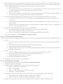 2
2