Theoretical Computer Science Cheat Sheet Page 3
ADVERTISEMENT
 1
1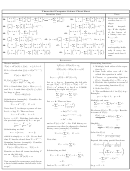 2
2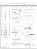 3
3 4
4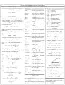 5
5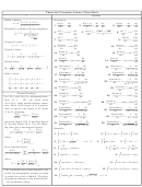 6
6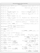 7
7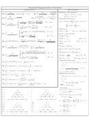 8
8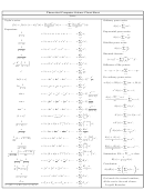 9
9 10
10Theoretical Computer Science Cheat Sheet
√
√
1+
5
1
5
ˆ φ =
π ≈ 3.14159,
e ≈ 2.71828,
γ ≈ 0.57721,
≈ 1.61803,
≈
φ =
.61803
2
2
i
i
2
p
General
Probability
i
1
2
2
Continuous distributions: If
Bernoulli Numbers (B
= 0, odd i = 1):
i
b
1
1
1
2
4
3
B
= 1, B
=
, B
=
, B
=
,
0
1
2
4
2
6
30
Pr[a < X < b] =
p(x) dx,
1
1
5
B
=
, B
=
, B
=
.
3
8
5
6
8
10
a
42
30
66
then p is the probability density function of
Change of base, quadratic formula:
4
16
7
√
X. If
2
b ±
log
x
b
4ac
5
32
11
a
Pr[X < a] = P (a),
log
x =
,
.
b
log
b
2a
6
64
13
a
then P is the distribution function of X. If
Euler’s number e:
7
128
17
P and p both exist then
1
1
1
1
+ · · ·
e = 1 +
+
+
+
a
8
256
19
2
6
24
120
P (a) =
p(x) dx.
n
x
x
9
512
23
∞
lim
1 +
= e
.
n
n→∞
Expectation: If X is discrete
10
1,024
29
n
n+1
1
1
1 +
< e < 1 +
.
n
n
E [g(X)] =
g(x) Pr[X = x].
11
2,048
31
e
11e
1
n
1
x
12
4,096
37
1 +
= e
+
O
.
2
3
n
2n
24n
n
If X continuous then
∞
∞
13
8,192
41
Harmonic numbers:
E [g(X)] =
g(x)p(x) dx =
g(x) dP (x).
14
16,384
43
3
11
25
137
49
363
761
7129
∞
∞
1,
,
,
,
,
,
,
,
, . . .
2
6
12
60
20
140
280
2520
15
32,768
47
Variance, standard deviation:
2
2
16
65,536
53
VAR[X] = E [X
]
E [X]
,
ln n < H
< ln n + 1,
n
17
131,072
59
1
σ =
VAR[X].
H
= ln n + γ + O
.
n
n
18
262,144
61
For events A and B:
Pr[A ∨ B] = Pr[A] + Pr[B]
Pr[A ∧ B]
Factorial, Stirling’s approximation:
19
524,288
67
Pr[A ∧ B] = Pr[A] · Pr[B],
. . .
1, 2, 6, 24, 120, 720, 5040, 40320, 362880,
20
1,048,576
71
iff A and B are independent.
21
2,097,152
73
√
n
n
1
Pr[A ∧ B]
n! =
2πn
1 + Θ
.
22
4,194,304
79
e
n
Pr[A|B] =
Pr[B]
23
8,388,608
83
Ackermann’s function and inverse:
For random variables X and Y :
24
16,777,216
89
j
2
i = 1
E [X · Y ] = E [X] · E [Y ],
a(i, j) =
a(i
1, 2)
j = 1
25
33,554,432
97
1)) i, j ≥ 2
if X and Y are independent.
a(i
1, a(i, j
26
67,108,864
101
α(i) = min{j | a(j, j) ≥ i}.
E [X + Y ] = E [X] + E [Y ],
27
134,217,728
103
E [cX] = c E [X].
Binomial distribution:
28
268,435,456
107
Bayes’ theorem:
n
29
536,870,912
109
k
n k
Pr[X = k] =
p
q
,
q = 1
p,
Pr[B|A
] Pr[A
]
k
i
i
|B] =
Pr[A
.
30
1,073,741,824
113
i
n
Pr[A
] Pr[B|A
]
n
j
j
j=1
n
31
2,147,483,648
127
k
n k
E [X] =
k
p
q
= np.
Inclusion-exclusion:
k
32
4,294,967,296
131
n
n
k=1
Pr
X
=
Pr[X
] +
Poisson distribution:
i
i
Pascal’s Triangle
λ
k
e
λ
i=1
i=1
1
Pr[X = k] =
,
E [X] = λ.
n
k
k!
k+1
( 1)
Pr
X
.
1 1
i
Normal (Gaussian) distribution:
j
k=2
i
<···<i
j=1
i
1 2 1
k
1
2
2
(x µ)
√
/2σ
p(x) =
e
,
E [X] = µ.
Moment inequalities:
1 3 3 1
2πσ
1
Pr |X| ≥ λ E [X] ≤
The “coupon collector”: We are given a
,
1 4 6 4 1
λ
random coupon each day, and there are n
1 5 10 10 5 1
1
E [X] ≥ λ · σ ≤
different types of coupons. The distribu-
Pr X
.
2
λ
1 6 15 20 15 6 1
tion of coupons is uniform. The expected
Geometric distribution:
1 7 21 35 35 21 7 1
number of days to pass before we to col-
k 1
Pr[X = k] = pq
,
q = 1
p,
lect all n types is
1 8 28 56 70 56 28 8 1
∞
1
nH
.
k 1
1 9 36 84 126 126 84 36 9 1
n
E [X] =
kpq
=
.
p
1 10 45 120 210 252 210 120 45 10 1
k=1
ADVERTISEMENT
0 votes
Related Articles
Related forms


Related Categories
Parent category: Education