Stat 110 - Cheat Sheet Page 4
ADVERTISEMENT
1. Cauchy-Schwarz:
X, Y
r.v.’s with finite variance.
Recurrent state: starting at that state, will return with
2
2
E[XY ]
E[X
]E[Y
]
probability 1. If the chain is irreducible, all states are
recurrent.
2. Jensen’s: X r.v. and g a convex ( or concave) func-
Transient state: not recurrent; starting at that state, will
tion. E[g(X)]
g(E[X]) ( or E[g(X)]
g(E[X])). e.g.
2
2
eventually leave and never return.
E[X
]
E[X]
and E[log(X)]
log E[X]
Period of state i: gcd of the possible numbers of steps
E[ X ]
3. Markov: X r.v. and a > 0. P ( X
a)
a
it can take to return to i when starting at i. Aperiodic
2
state: state with period 1. Aperiodic chain: all states
4. Chebyshev: X r.v. with mean µ and variance σ
. P ( X
2
have period 1.
σ
µ
a)
.
2
a
Stationary Distribution:
Law of Large Number (LLN) Let X
, X
, X
, . . . be i.i.d.
1
2
3
random variables drawn from some distribution with mean
Stationary distribution is probability row vector s satis-
µ = E[X
] for all i, then
i
fying sQ = s. Assuming irreducibility and aperiodicity:
X
+
+ X
1
n
– s is unique.
¯ S
lim
= lim
= µ
n
n
n
n
– s
is long-run probability of being at state i :
i
m
lim
Q
is a matrix whose rows are all s.
The Central Limit Theorem (CLT) Let Y be the sum of n,
n
for some large n, i.i.d. random variables drawn from some
– Expected time to return to i, starting at i, is 1/s
.
i
distribution with mean E[Y ] = µ
and variance var(Y ) =
Y
2
Reversibility:
σ
, then
Y
.
2
Y
N (µ
, σ
),
Y
Y
Reversible chain: there exists s satisfying s
q
= s
q
i
ij
j
ji
.
for all i and j. Then s is the stationary distribution,
where
denotes is approximately distributed. When we use
assuming the entries sum to 1.
the CLT we usually have that Y
= X
+
+ X
or Y
=
1
1
n
2
¯ X
1
=
(X
+
+ X
). Specifically if we assume that each
n
1
n
n
Important cases of reversibility:
2
X
has mean µ
and variance σ
then
i
X
X
– Columns of Q sum to 1:s is uniform over all states.
.
2
Y
N (nµ
, nσ
),
1
X
(Note that this applies to all symmetric transition
X
2
σ
matrices.)
.
= ¯ X
X
Y
N µ
,
.
2
n
X
n
– Random walk on undirected network: s is propor-
tional to degree sequence.
Markov Condition:
Metropolis algorithm:
Markov chain X
, X
, X
, . . . on state space 1, . . . , M
0
1
2
satisfies the Markov condition
Start with desired distribution s and an arbitrary chain
with transition matrix P .
P (X
= j X
= i
, X
= i
, . . . , X
= i
, X
= i)
n+1
0
0
1
1
n 1
n 1
n
Define new chain whose transitions are
= P (X
= j X
= i)
n+1
n
s
p
j
ji
q
= p
min
, 1
ij
ij
Only today’s information matters for predicting tomor-
s
p
i
ij
row; additional information about the past is redundant
s p
given today’s information. Given the present, the past
p
is the proposal probability, and min
, 1 is the
ij
s p
and future are conditionally independent.
acceptance probability.
Transition Matrix:
The new chain satisfies s
q
= s
q
, hence has station-
i
ij
j
ji
ary distribution s.
The (i, j) entry of transition matrix Q gives the prob-
ability of going from state i to state j in one step:
g
= q
= P (X
= j X
= i).
i
j
ij
n+1
n
(m)
m
Q
is the m-step transition matrix: q
= P (X
=
n+m
ij
j X
= i).
n
If v is the row vector encoding the PMF of X
, such that
0
n
P (X
= i) = v
, then the PMF of X
is vQ
.
0
i
n
Irreducible chain: can get from any state to any other
state in a finite number of steps.
Classification of States:
4
ADVERTISEMENT
0 votes
Related Articles
Related forms
Related Categories
Parent category: Education
 1
1 2
2 3
3 4
4