Sales Forecast Of An Automobile Industry Page 3
ADVERTISEMENT
 1
1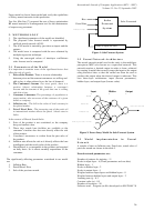 2
2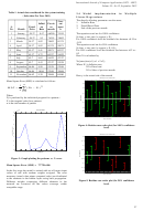 3
3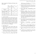 4
4International Journal of Computer Applications (0975 – 8887)
Volume 53– No.12, September 2012
Table 1. Actual data considered for the system training
Model implementation in Multiple
2.4
( Sales data For Year 2011)
Linear Regressions
The directly affecting parameters are the same:
Curr
1.
Inflation Rate
Inflati
Previo
ent
2.
Petrol/Diesel Price
S.
Petrol
on
us
mont
3.
Sale of the previous month.
No.
Month
Price
Rate
month
h
1
January
58.37
9.47
66290
74355
The equations used are for 100% confidence
[b, bint, r, rint, stats] = regress(y, X);
2
Februray
58.37
9.3
74355
74802
For 100% confidence level the residuals lies between +0.35 to
3
March
58.37
8.82
74802
81375
-0.35
The equations used are for 50% confidence
4
April
58.37
8.82
81375
59971
[b, bint, r, rint, stats] = regress(y, X, 0.5);
5
May
63.37
9.41
59971
65237
For 50% confidence level the residuals lies between +0.2 to -
0.2
6
June
63.37
8.72
65237
54422
Here X is calculated by
7
July
63.7
8.62
54422
47127
X=[ones(size(x1)) x1 x2 x3];
8
August
63.7
8.43
47127
53539
Where X1 is Inflation rate,
9
September 66.84
8.99
53539
57049
X2 is Petrol rate
X3 is Sales of previous month
10
October
66.84
10.06
57049
35868
11
November 66.42
9.39
35868
61080
Here y is the actual sale of the month
Residual Case Order Plot
Mean Square Error (MSE) is calculated as follows:
0.3
n
1
2
MSE
(
D
F
)
t
t
0.2
n
t
1
0.1
Where
D
is predicted by the individual program for a pattern t
0
t
F
is the targeted value for a pattern t
t
-0.1
n is the total number of pattern
-0.2
-3
Plot of MSE
x 10
9
-0.3
8
1
2
3
4
5
6
7
8
9
10
11
Case Number
7
6
Figure 4: Residue case order plot (for 100% confidence
level)
5
4
Residual Case Order Plot
0.2
3
2
0.15
1
0.1
0
0.05
1
2
3
4
5
6
7
8
9
10
11
patterns
0
Figure 3: Graph plotting the patterns vs. % error
-0.05
-0.1
Mean Square Error (MSE) = 7.7728e-006
-0.15
In the first stage the model is trained with set of known input
-0.2
values of sale with random weights assigned. The error
1
2
3
4
5
6
7
8
9
10
11
Case Number
measures (actual value minus computed value) are distributed
to the elements in the hidden layers using back propagation.
Figure 5: Residue case order plot (for 50% confidence
Different weights connecting different elements in the
level)
network are corrected till the values converge within
acceptable range.
27
ADVERTISEMENT
0 votes
Related Articles
Related forms


Related Categories
Parent category: Financial