Lab 8: Excel Functions And Formulas Cheat Sheet Page 3
ADVERTISEMENT
 1
1 2
2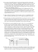 3
312. Use a series of nested IF functions to turn the percentage grade into a letter grade.
The IF function takes 3 arguments: a logical test, a value to use if the test is true, and
a value to use if it is false. The function IF(H3>=90,”A”,”B”) would give the value
“A” if the contents of H3 were greater than or equal to 90, “B” if not. All you have to
do to get the whole range is plug another test in instead of the “B” and work your way
down to “F” (let’s skip the +’s and -’s):
=IF(H9>=90,"A",IF(H9>=80,"B",IF(H9>=70,"C",IF(H9>=60,"D","F"))))
Take a minute to think about this formula and figure out how it works. It isn’t really
as complicated as it looks, it’s just that the 3rd argument of each IF function is the
value returned from the next IF function, i.e. if H3 is less than 90, it checks to see if it
is greater than 80 or not, etc.
13. Apply conditional formatting to the letter grades so that A’s are highlighted in blue
and F’s in red (if you don’t have any A’s or F’s, fudge a few grades so you will).
14. Browse through your students using Data Filter to see who got A’s, B’s, etc. Choose
Autofilter from the menu, and then you can use the little arrows at the top of each
column to filter the list according to which grades you want to look at. When you are
done, choose All from the list of possibilities to show all the records again.
15. To finish up, you want to tabulate how many A’s, B’s, C’s, etc. your students got.
For this you will use the Data Table command. The table needs to be set up in
advance, though. Choose a location out of the way below your grades. Type the
grades A through F in a column one below the other. In the next column to the right,
enter a Countif function (counts the number of cells meeting a criterion). The first
argument of the function should be the range of cells that contain the grades. The
second argument should be a cell out of the way on the side that you can type a grade
into (G10 in my example). Finally, select the two columns of the table including the
cell above the A, the formula, and the block of cells containing grades and blank cells
to their right. Now do the Data Table command, give the cell that your formula refers
to (G10 in my example) for the “column input cell” (leave the row input blank – you
would use both if you had a 2-dimensional table) and press “OK”. Excel should fill in
the rest of the table for you.
G10
=COUNTIF(J1:J7,G10)
A
A
B
C
D
E
16. Finally, make sure your name is on your spreadsheet somewhere (insert another row at
the top if you need to). Use Print preview to be sure it will fit on one page and adjust
whatever you need to to make it fit, then print it and hand it in with the diskette.
ADVERTISEMENT
0 votes
Related Articles
Related forms


 Tool Bar And Windows Cheat Sheet")

Related Categories
Parent category: Education