Inventory Control Guide Page 10
ADVERTISEMENT
 1
1 2
2 3
3 4
4 5
5 6
6 7
7 8
8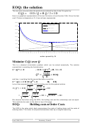 9
9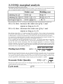 10
10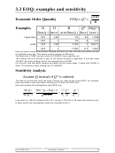 11
11 12
12 13
13 14
14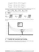 15
15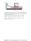 16
16 17
17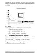 18
18 19
19 20
20 21
21 22
22 23
23 24
24 25
25 26
26 27
27 28
28 29
29 30
30 31
31 32
32 33
33 34
34 35
35 36
36 37
37 38
38 39
39 40
403.2 EOQ: marginal analysis
Here we will analyze this EOQ solution.
The EOQ was found assuming continuous Q values. If we assume Q to take discrete values
only, a marginal analysis is needed. Let's see that it leads to a similar formula.
Order cost
Holding cost
ordering by Q
O D / Q
H Q / 2
ordering by (Q+1) O D / ( Q + 1)
H (Q +1) / 2
∆=C(Q)-C(Q+1)
O D / Q(Q+1)
- H / 2
We proceed from Q to Q+1, as long as increasing the order size decreases the total cost.
If ∆ > 0, then increase the order size Q by 1 and
repeat as long as ∆ > 0.
If ∆ < 0, then decrease the order size Q by 1 and
repeat as long as ∆ < 0.
We will thus stop when ∆ ≈ 0, that is when Q(Q+1)≈2OD/H. This is close to the expression
Q*Q≈2OD/H which gives the EOQ. The difference between the formulas results from the kind
of differentiation: a continuous derivative for the EOQ and a discrete derivative here above.
It is important to understand and to be able to apply the principle of the marginal analysis. The
idea is to compare two neighboring solutions, for example Q and Q+1.
If Q+1 is better then we will successively try Q+2, Q+3,... as long as some gain is observed.
On the other hand, if Q is better than Q=1, then we will successively try Q-1, Q-2,..., again as
long as the cost function decreases. With this marginal approach, a minimum is always
reached. However, this minimum could be local. It is global if the function does not admit local
minima. This is the case here. Indeed, the plot of the total cost function clearly shows that the
cost function has a unique (global) minimum.
BEF
unit
unit year
= k
Finding back EOQ:
units
1
year
BEF
Note that if you forget the formula, you can almost find it back using the units. You are looking
for Q (in items) and you have D (in item/year), O (in money) and H (in money / (year.item)).
You quickly find that the simplest formula of the form Q=f(O,D,H) which keeps consistent units
is the Q=sqrt(OD/H). Unfortunately, it does not give you the constant k = sqrt(2).
2OD
EOQ = Q* =
Economic Order Quantity
H
Because we order by lots of size Q*, the average inventory level is Q*/2. This average stock is
usually referred to as the cycle stock.
Cycle stock :
Q*/2
Prod 2100-2110
Inventory Control
9
ADVERTISEMENT
0 votes
Related Articles
Related forms


Related Categories
Parent category: Education