Inventory Control Guide Page 13
ADVERTISEMENT
 1
1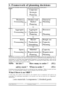 2
2 3
3 4
4 5
5 6
6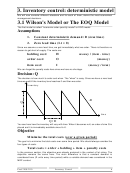 7
7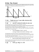 8
8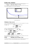 9
9 10
10 11
11 12
12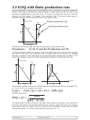 13
13 14
14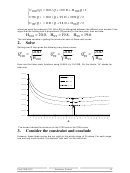 15
15 16
16 17
17 18
18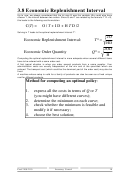 19
19 20
20 21
21 22
22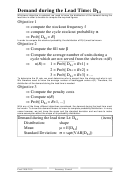 23
23 24
24 25
25 26
26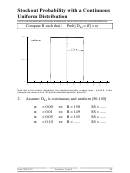 27
27 28
28 29
29 30
30 31
31 32
32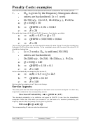 33
33 34
34 35
35 36
36 37
37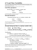 38
38 39
39 40
403.5 EOQ with finite production rate
Here we describe a model where the production rate is assumed to be finite (instead of
infinite). This means that when an order is started, it takes some time for the order to be
performed (independently of the lead time). The items are produced not all at once but
regularly with some speed. This speed is the production rate. This model makes sense in
production systems that are almost continuous (e.g. glass sector).
Inventory
Infinite production rate
T 1
Finite production rate
-D
Q
Pr
T=Q/D
Compared to Wilson's model, the only new parameter is the production rate.
Parameters:
D; H, O and the Production rate Pr
The finite production speed can be seen as an advantage since we receive the items regularly
over time. At the limit, if the production rate is exactly equal to the demand, the average
inventory vanishes! In that case, each unit is produced when needed and not before. In all
cases, the average inventory is smaller compared to that with an infinite production rate.
Inventory
T 1
T 1
Y
-D
Q
Pr
-D
Pr-D
time
T
T
The average inventory amounts to half the height of the bold triangle. What is its height? It is:
Q - Y = Q - D×T1 = Q - D×Q/Pr= Q(1-D/Pr).
C(Q) =
O (D / Q) + I D + H (1 - D/Pr) Q/2
Solving over Q gives:
2OD
EOQ = Q* =
−
H(1 D / Pr)
It is always good to check a formula. In this case, three checks are possible. First, replace PR
by infinite. The result is the classical EOQ formula. Second, replace PR by 2D (you produce
twice quicker than you need). You can check that the average inventory level is indeed
reduced by a factor 1/2. Third on could check the formula for Pr = D.
Prod 2100-2110
Inventory Control
12
ADVERTISEMENT
0 votes
Related Articles
Related forms


Related Categories
Parent category: Education