Inventory Control Guide Page 7
ADVERTISEMENT
 1
1 2
2 3
3 4
4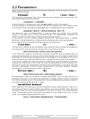 5
5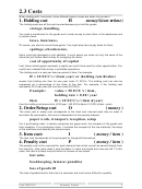 6
6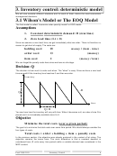 7
7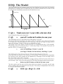 8
8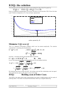 9
9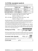 10
10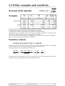 11
11 12
12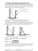 13
13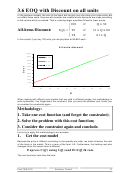 14
14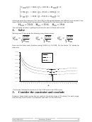 15
15 16
16 17
17 18
18 19
19 20
20 21
21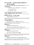 22
22 23
23 24
24 25
25 26
26 27
27 28
28 29
29 30
30 31
31 32
32 33
33 34
34 35
35 36
36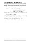 37
37 38
38 39
39 40
403. Inventory control: deterministic model
We will now consider different situations and for each of them, derive the most economical
management decisions.
3.1 Wilson's Model or The EOQ Model
The first model is called: "economic order quantity model" or EOQ model.
Assumptions
1.
Constant deterministic demand: D (item/time)
2.
Zero lead time (Lt = 0)
Since we assume a zero lead time, we get immediately what we order. There is therefore no
reason to get short of supply. The costs are:
holding cost:
H
money / (item . time)
order cost:
O
(money)
item cost:
I
(money / item)
We can forget the penalty costs here since we have no shortage.
Decision: Q
The decision is how much to order and when. The "when" is easy. Since we have a zero lead
time we wait till the inventory level reaches 0 and then we order.
Inventory
-D
Q
time
Q / D
You see here how the inventory will vary with time. When it becomes null, an order of size Q is
placed and it is immediately available since Lt=0.
Objective
Minimize the total costs (over a given period)
The goal is to minimize the total costs over some time period. We should always consider the
four types of costs.
Total costs = order + holding + item + penalty costs
In the previous section, this objective was already analyzed in the context of lot sizing. The
objective remains the same here. The main difference is that a constant demand is
considered here (D units every time period) while a variable demand was considered in the
MRP context.
Prod 2100-2110
Inventory Control
6
ADVERTISEMENT
0 votes
Related Articles
Related forms


Related Categories
Parent category: Education