Inventory Control Guide Page 30
ADVERTISEMENT
 1
1 2
2 3
3 4
4 5
5 6
6 7
7 8
8 9
9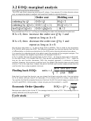 10
10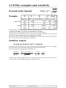 11
11 12
12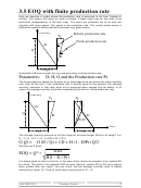 13
13 14
14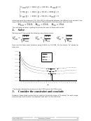 15
15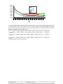 16
16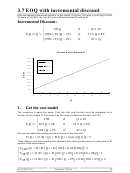 17
17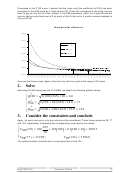 18
18 19
19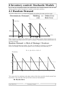 20
20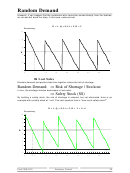 21
21 22
22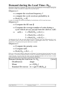 23
23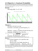 24
24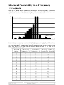 25
25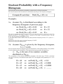 26
26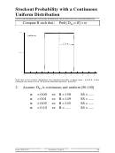 27
27 28
28 29
29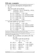 30
30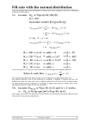 31
31 32
32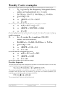 33
33 34
34 35
35 36
36 37
37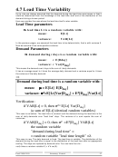 38
38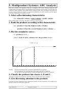 39
39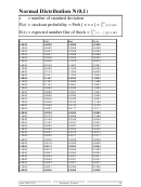 40
40Fill rate: examples
Here we will consider different examples and show how to determine the reorder point R.
1.
D
is given by the frequency histogram above
Lt
Q = 30
backorder model: β =( Q -n( R ))/ Q
n( R ) =
1 Prob[ D
= R +1] + 2Prob[ D
= R +2]+
Lt
Lt
3 Prob[ D
= R +3] + ...
Lt
β = 1.00
R = 23
n(R)=0
β = 29.99/30=0.9997
R = 22
n(R)=0.01
β = 29.97/30=0.9990
R = 21
n(R)=0.03
β =
R = 15
n(R)=1.08
β =
R = 6
n(R) =
Here we consider the same situation except that the sales are assumed to be lost.
lost sales model: Q / ( Q + n( R ) )
β = 1.00
R = 23
n(R)=0
β = 30/30.01=0.9997
R = 22
n(R)=0.01
β = 30/30.03=0.9990
R = 21
n(R)=0.03
β =
R = 15
n(R)=1.08
β =
R = 6
n(R) =
Do not try to compare the two models in terms of fill rate because they correspond to
situations which are different in the reality and with different cycle lengths.
Note however the role played by the lot size Q. If we choose a lot size twice larger, we can
allow twice as many lost (or backordered) sales while keeping the same fill rate.
Note also the difference between α and β: α is a probability and is computed per cycle, β is a
percentage and it is independent of the time.
2.
Assume: D
is continuous and uniform [50-150]
Lt
Q = 100
backorder model: β =( Q -n( R ))/ Q
∞
=
−
n( )
R
(
x
R f
)
( )
x dx
D
R
Lt
β = 1.00
R = 150
n(R)=0
β = 0.99875
R = 145
n(R)=0.125
β = 0.995
R = 140
n(R)=0.5
β =
R = 100
n(R)=12.5
β =
R = 50
n(R)=
Prod 2100-2110
Inventory Control
29
ADVERTISEMENT
0 votes
Related Articles
Related forms


Related Categories
Parent category: Education