Inventory Control Guide Page 23
ADVERTISEMENT
 1
1 2
2 3
3 4
4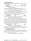 5
5 6
6 7
7 8
8 9
9 10
10 11
11 12
12 13
13 14
14 15
15 16
16 17
17 18
18 19
19 20
20 21
21 22
22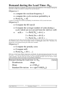 23
23 24
24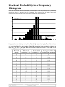 25
25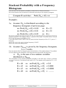 26
26 27
27 28
28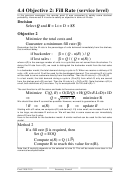 29
29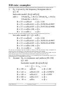 30
30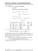 31
31 32
32 33
33 34
34 35
35 36
36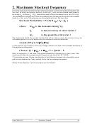 37
37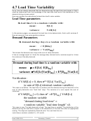 38
38 39
39 40
40Demand during the Lead Time: D
Lt
Whichever objective is selected, we need to know the distribution of the demand during the
lead time in order to be able to compute the required figures.
Objective 1
compute the stockout frequency f
compute the cycle stockout probability α
Prob[ D
> R]
Lt
In order to compute this stockout probability, the distribution of D(Lt) must be known.
Objective 2
Compute the fill rate β
Compute the average number of units during a
cycle which are not served from the shelves: n(R)
1 × Prob[ D
n(R) =
= R+1] +
Lt
2 × Prob[ D
= R+2] +
Lt
3 × Prob[ D
= R+3] + ...
Lt
To determine the fill rate, we must determine who is served from the shelve and who is not.
We therefore need to know the average number of backlogged orders n(R). Therefore, the
distribution of the demand during the lead time is needed.
Objective 3
Compute the penalty costs
Compute n(R)
Prob[ D
= R+1, ...]
Lt
With any of the three different objectives considered, the demand during the lead time must
be known. To know this demand means to know its complete probability distribution. In many
cases however, we just know the mean and the standard deviation and we have to make
some assumption about the shape of its probability distribution.
Demand during the lead time Lt: D
(items)
Lt
Distribution:
shape
µ = E[D
Mean:
]
Lt
Standard Deviation: σ = sqrt(VAR[D
])
Lt
Prod 2100-2110
Inventory Control
22
ADVERTISEMENT
0 votes
Related Articles
Related forms


Related Categories
Parent category: Education