Inventory Control Guide Page 12
ADVERTISEMENT
 1
1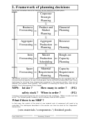 2
2 3
3 4
4 5
5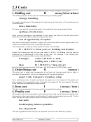 6
6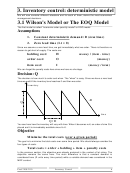 7
7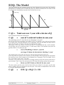 8
8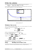 9
9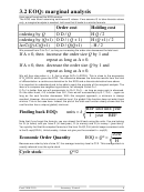 10
10 11
11 12
12 13
13 14
14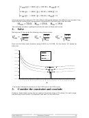 15
15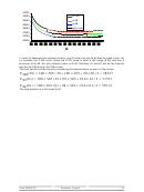 16
16 17
17 18
18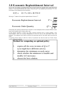 19
19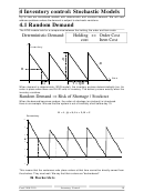 20
20 21
21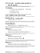 22
22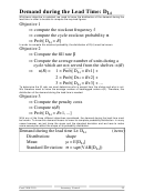 23
23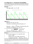 24
24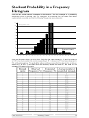 25
25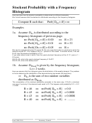 26
26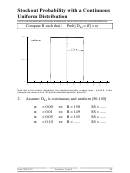 27
27 28
28 29
29 30
30 31
31 32
32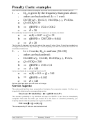 33
33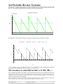 34
34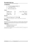 35
35 36
36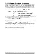 37
37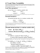 38
38 39
39 40
403.4 EOQ with positive Lead time.
Let us consider again the EOQ model but let us assume that the time between an order is
placed and the same order is received is nonnull.
Assumptions:
deterministic
1.
Constant
demand: D ( item / time )
2. Positive lead time (Lt > 0)
We will see that the costs do not change. Shortages are still avoided.
Since the costs do not change, we will still order by Q* but we will order earlier.
Q = EOQ = Q* = 2OD / H
How much to order:
When to order :
Lt before the inventory vanishes or
• • • •
When the inventory position
• • • •
reaches the reorder point R = Lt D
Specifying that an order must be launched Lt days before the inventory vanishes is not very
convenient. It is easier to specify the order point as an inventory value: order when there are
only R units left.
Inventory
Q
-D
R
time
Lt
Here are two examples which show that R could become a virtual inventory.
D=365 items /year
Q* = 6
Lt = 3 days
R = 3 items
D=365 items /year
Q* = 6
Lt = 10 days
R= 10 items
In the second example, one should order when the inventory reaches the value 10 while the
inventory varies between 6 and 0....That's why we need the notion of inventory position.
Inventory position = inventory on-hand + inventory on-order
A positive lead time leads to the notion of pipeline stock or pipeline inventory. This is the
amount of items in transit. Holding costs could be due for this inventory.
Pipeline stock:
Lt D
(items)
Pipeline cost:
Lt D H
(money / time)
If the demand is 365 items/year, and if the lead time is 10 days, the pipeline stock is 10 items.
With a holding cost H=20/(item.year), this leads to a pipeline cost of 200/year.
Positive Lead time
Pipeline Stock
As long as the demand is known and constant, the existence of a lead time does not change
the problem. It does only shift the time at which an order is placed.
Prod 2100-2110
Inventory Control
11
ADVERTISEMENT
0 votes
Related Articles
Related forms


Related Categories
Parent category: Education