What-If Analysis, Charting, And Working With Large Worksheets Page 43
ADVERTISEMENT
 1
1 2
2 3
3 4
4 5
5 6
6 7
7 8
8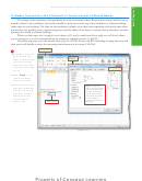 9
9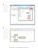 10
10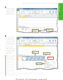 11
11 12
12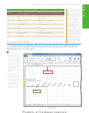 13
13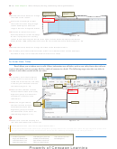 14
14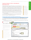 15
15 16
16 17
17 18
18 19
19 20
20 21
21 22
22 23
23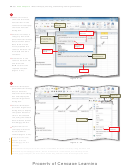 24
24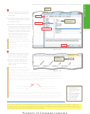 25
25 26
26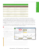 27
27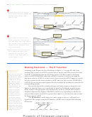 28
28 29
29 30
30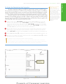 31
31 32
32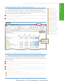 33
33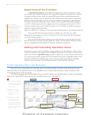 34
34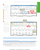 35
35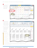 36
36 37
37 38
38 39
39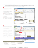 40
40 41
41 42
42 43
43 44
44 45
45 46
46 47
47 48
48 49
49 50
50 51
51 52
52 53
53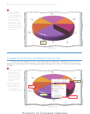 54
54 55
55 56
56 57
57 58
58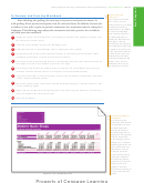 59
59 60
60 61
61 62
62 63
63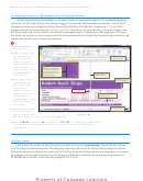 64
64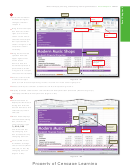 65
65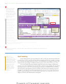 66
66 67
67 68
68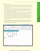 69
69 70
70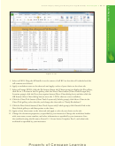 71
71 72
72 73
73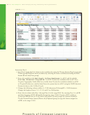 74
74 75
75 76
76 77
77 78
78 79
79 80
80 81
81 82
82 83
83 84
84 85
85 86
86 87
87What-If Analysis, Charting, and Working with Large Worksheets
Excel Chapter 3
EX 179
3
•
With the mouse
pointer still a block
plus sign with a
paintbrush, drag
through the range
A25:I25 to assign the
format of the source
cell, A13 in this case,
to the destination
range, A25:I25 in
this case.
•
Press the ESC key
format copied to range
A25:H25 and Currency
to stop the format
style applied to range
painter.
B25:I25
•
Apply the Currency
style to the range
B25:H25 to cause the
cells in the range
to appear with a
fl oating dollar sign
and two decimal
places and then scroll
Figure 3 – 49
the worksheet so that
Other Ways
column A is displayed (Figure 3 –49).
1. Click Copy button
(Home tab | Clipboard
Why does the Currency style need to be reapplied to the range B25:H25?
group), select cell, click
Paste button arrow
Sometimes, the use of the format painter results in unintended outcomes. In this case, the
(Home tab | Clipboard
changing of the background fi ll color and font color for the range B25:H25 resulted in the
group), click Formatting
loss of the Currency style because the format being copied did not included the Currency
icon on Paste gallery
style. Reapplying the Currency style to the range results in the proper number style, fi ll color,
2. Right-click cell, click
Copy, right-click cell,
and font color.
click Formatting icon on
shortcut menu
To Format the What-If Assumptions Table
and Save the Workbook
Painting a Format to
The last step to improving the appearance of the worksheet is to format the
Nonadjacent Ranges
Double-click the Format
What-If Assumptions table in the range A1:B8. The specifi cations in Figure 3– 40 on page
Painter button (Home tab
EX 173 require an 8-point italic underlined font for the title in cell A1 and 8-point font in
| Clipboard group) and
the range A2:B8. The following steps format the What-If Assumptions table.
then drag through the
nonadjacent ranges to
1
+
Press
to select cell A1.
CTRL
HOME
paint the formats to the
ranges. Click the Format
2
Click the Font Size button arrow (Home tab | Font group) and then click 8 in the Font Size
Painter button (Home
list to decrease the font size of the selected cell.
tab | Clipboard group) to
deactivate it.
3
Click the Italic button (Home tab | Font Group) and then click the Underline button
(Home tab | Font group) to italicize and underline the text in the selected cell.
4
Select the range A2:B8, click the Font Size button arrow (Home tab | Font group) and
then click 8 in the Font Size list to apply a smaller font size to the selected range.
5
Select the range A1:B8 and then click the Fill Color button (Home tab | Font group) to
apply the most recently used background color to the selected range.
ADVERTISEMENT
0 votes
Related Articles
Related forms


Related Categories
Parent category: Education