What-If Analysis, Charting, And Working With Large Worksheets Page 76
ADVERTISEMENT
 1
1 2
2 3
3 4
4 5
5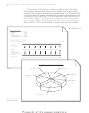 6
6 7
7 8
8 9
9 10
10 11
11 12
12 13
13 14
14 15
15 16
16 17
17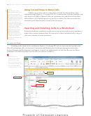 18
18 19
19 20
20 21
21 22
22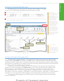 23
23 24
24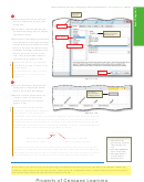 25
25 26
26 27
27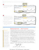 28
28 29
29 30
30 31
31 32
32 33
33 34
34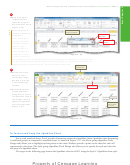 35
35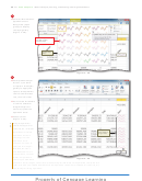 36
36 37
37 38
38 39
39 40
40 41
41 42
42 43
43 44
44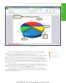 45
45 46
46 47
47 48
48 49
49 50
50 51
51 52
52 53
53 54
54 55
55 56
56 57
57 58
58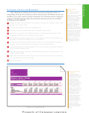 59
59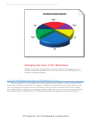 60
60 61
61 62
62 63
63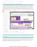 64
64 65
65 66
66 67
67 68
68 69
69 70
70 71
71 72
72 73
73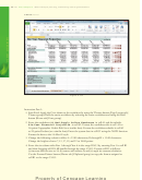 74
74 75
75 76
76 77
77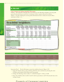 78
78 79
79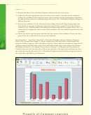 80
80 81
81 82
82 83
83 84
84 85
85 86
86 87
87EX 212
Excel Chapter 3
What-If Analysis, Charting, and Working with Large Worksheets
continued
In the Lab
aa. Year 1 Income Taxes (cell B18): If Year 1 Operating Income is less than 0, then Year 1 Income
Taxes equal 0; otherwise Year 1 Income Taxes equal 45% * Year 1 Operating Income
or =IF(B17 < 0, 0, 45%*B17)
bb. Copy cell B18 to the range C18:G18.
cc. Year 1 Net Income (cell B19) = Year 1 Operating Income − Year 1 Income Taxes or = B17-B18
dd. Copy cell B19 to the range C19:G19.
ee. In cell H4, insert a Sparkline Column chart (Insert Tab| Sparklines group) for cell range B4:G4
ff. Repeat step ee for the ranges H5:H6, H8:H15, and H17:H19
9. Change the background colors as shown in Figure 3 –87. Use Teal, Accent 3, Lighter 40% for the
background colors.
10. Zoom to: (a) 200%; (b) 75%; (c) 25%; and (d) 100%.
11. Change the document properties, as specifi ed by your instructor. Change the worksheet header
with your name, course number, and other information as specifi ed by your instructor. Save
the workbook using the fi le name, Lab 3-1 Med Supply Online Warehouse Six-Year Financial
Projection.
12. Preview the worksheet. Use the Orientation button (Page Layout tab | Page Setup group) to fi t
the printout on one page in landscape orientation. Preview the formulas version (ctrl+`) of the
worksheet in landscape orientation using the Fit to option. Press ctrl +` to instruct Excel to display
the values version of the worksheet. Save the workbook again and close the workbook.
13. Submit the workbook as specifi ed by your instructor.
Instructions Part 2:
1. Start Excel. Open the workbook Lab 3-1 Med Supply Online Warehouse Six-Year Financial
Projection.
2. Use the nonadjacent ranges B3:G3 and B19:G19 to create a 3-D Cylinder chart. Draw the chart
by clicking the Column button (Insert tab | Charts group). When the Column gallery is displayed,
click the Clustered Cylinder chart type (column 1, row 3). When the chart is displayed, click the
Move Chart button to move the chart to a new sheet.
3. Select the legend on the right side of the chart and delete it. Add the chart title by clicking the
Chart Titles button (Chart Tools Layout tab | Labels group). Click Above Chart in the Chart Title
gallery. Format the chart title as shown in Figure 3–88.
4. To change the color of the cylinders, click one of the cylinders and use the Shape Fill button (Chart
Tools Format tab | Shape Styles group). To change the color of the wall, click the wall behind the
cylinders and use the Shape Fill button to change the chart wall color. Use the same procedure to
change the color of the base of the wall.
5. Rename the sheet tabs Six-Year Financial Projection and 3-D Cylinder Chart. Rearrange the sheets
so that the worksheet is leftmost and color their tabs as shown in Figure 3–88.
6. Click the Six-Year Financial Projection tab to display the worksheet. Save the workbook using the
same fi le name (Lab 3-1 Med Supply Online Warehouse Six -Year Financial Projection) as defi ned
in Part 1. Submit the workbook as requested by your instructor.
ADVERTISEMENT
0 votes
Related Articles
Related forms


Related Categories
Parent category: Education